APPLICATION OF TIME SERIES ANALYSIS IN FINANCIAL ECONOMICS
In this blog, I will explain to you a few applications of Time Series Analysis in financial economics. But, before that let us understand what exactly a time series analysis and Data Analysis
Time Series Analysis
A time series is actually a sequence of data points recorded at regular intervals of time (yearly, quarterly, monthly, daily). Time series includes two types:
1. Univariate — involves a single variable
2. Multivariate — involves two or more variables
Let me present you with a list of examples of time series:
ü Monthly or daily precipitation of a region
ü Daily stock prices (opening, closing) over a period of years/days.
ü Monthly bike sales over a period of 3 years
ü Annual unemployment rate over a period of 10 years
Forecasting Time Series Data
The main objective of a Time Series Analysis is to develop a suitable model to describe the pattern or trend in data with more accuracy. However, forecasting a time series data predicts future outcomes based on the immediate past. Forecasting can be done for closing/opening the rate of stock on a daily basis, quarterly revenues of a company, etc., There are various models available in the literature to forecast the time series data. Some of them are:
- Autoregressive Integration Moving Average (ARIMA)
- Simple Moving Average (SMA)
- Exponential Smoothing (SES)
- Neural Network (NN)
- Linear Regression Models
- Logistic Regression
- Support Vector Machine
- Naive Bayes
- Hidden Markov
- VAR
- Gaussian Processes
Well, many complex models or techniques may be useful in certain cases to forecast time series data. They are:
· Neural Networks Autoregression (NNAR)
· RNN (Recurrent Neural Network)
· Generalized Autoregressive Conditional Heteroskedasticity (GARCH)


The performance of the time series models can be interpreted based on its error terms such as AIC, BIC, Mean Squared Error, etc. and it can be emphasized for forecasting.
The principle interest for every time series analysis is to split the original series into independent components. The decomposition of time series is much easy to forecast the individual regular patterns produced than from the actual series. Typically, time series are further split into three main components:
· Trend
· Seasonality
· Cycle


Applications of Time Series Forecasting:
Time series models usually used to forecast the stock’s performance, interest rate, weather, etc. In this post, we will look at a few situations where time series can be useful to forecast future outcomes.
Application 1:
In this example, we will look at the daily values of the data with the time factors available between 2010 and 2016 from the Yahoo Finance repository. I extracted the entire timeline for 4 related time series (SERIES A values and volumes, SERIES B values and volumes). Forecasting is done for SERIES A values based on the most recent trend (lags) of SERIES A volumes and SERIES B values and volumes. Apart from this, we make use of another dataset from Kaggle to forecast the market sentiment. The data involves top daily news headlines between 2008 and 2016.
The primary step in the time series analysis is that one should check whether the time series is approximately stationary and normalized. For this situation, RNN forecasting is used to predict the outcomes variable of interest that results in the inference of the future time evolution of the SERIES A values based on its past trends (including volumes) as well as the past trend of another SERIES B, and market sentiment.
Forecast future values of time series
It forecasts SERIES A values based on the most recent trend (lags) of SERIES A volumes, SERIES B values and volumes, and market sentiment using ARIMA model. The mean absolute error (MAE) is used to understand the trend in this graph and it is 10, 24, 14, 15 for each sample respectively. The following figure shows a comparison of 10-day forecast.


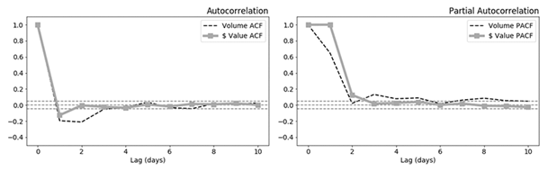
In a traditional regression data, dependent or response variable is influenced by a set of independent variables. The degree of dependence on previous outcomes varies for each case, and can be explained by (ACF) Auto Correlation Factor as given in below figure.
Figure: ACF and PACF Plots of SERIES A value and volume.


Looking at the ACF and PACF plots, one can choose proper values of the parameters in the model. The results from ARIMA model will look like:
Especially, from the results SERIES B values significantly influences the forecasting made for SERIES A. The market sentiment (s) does too but to a lower extent, and volumes are relatively insignificant for forecasting the SERIES A values with ARIMA.
Speak with our Statswork experts for time series forecasting to build the marketing strategy of financial organization.
Applications 2:
As a second example, we will look at the stock market data from 2016 from Kaggle and analyze the pattern of the data. The data involves stocks of top companies such as Facebook, Apple, Amazon, etc. Here is the trend of the daily closing price of stocks for the month of January.

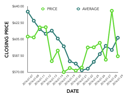
The following graph depicts the trend of price change for the month of January. This is often referred to as “momentum” in financial research.


Time series in financial economics are highly important to analyze the trend or pattern of the variable of interest using an appropriate model. The above example clearly depicts the trend in the price of the stock and this trend may be helpful in predicting future stock values using suitable models as mentioned earlier.
Application 3:
Lastly, let us look at a situation where the trend of the sales and tractor demand in the XYZ manufacturing company is to be analyzed. The company is interested in understanding the impact of marketing efforts on sales. In such a situation, finding the pattern of the sales and demand can be viewed using a well-known ARIMA model and predict the sales/demand for the upcoming years. In addition, the impact of the marketing effort can be studied using exogenous variables under the ARIMA model.
To sum up, there are various applications apart from these three that are available in our day-to-day life. However, many financial organization relies on time series forecasting to build their marketing strategy to meet the customer’s needs. Thus, a more proper model should be selected to analyze the pattern of financial data.
References
Dunning, T., & Friedman, E. (2015). Time Series Databases (1st ed.). California: O’Reilly Media.
Hyndman, R., & Athanasopoulos, G. (2017). Forecasting: Principles and Practice (2nd ed.)
Hyndman, R., & Khandakar, Y. (2008). Automatic time series forecasting: the forecast package for {R}. Journal of Statistical Software, 26(3), 1–22.
As a second example, we will look at the stock market data from 2016 from Kaggle and analyze the pattern of the data. The data involves stocks of top companies such as Facebook, Apple, Amazon, etc. Here is the trend of the daily closing price of stocks for the month of January.
.jpg)
Comments
Post a Comment